{cansim} and Data Visualization

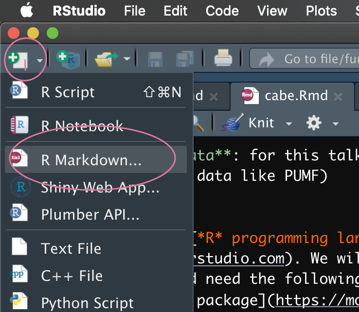
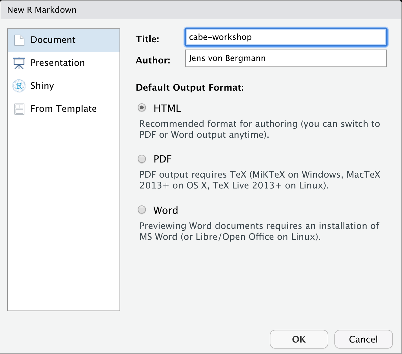
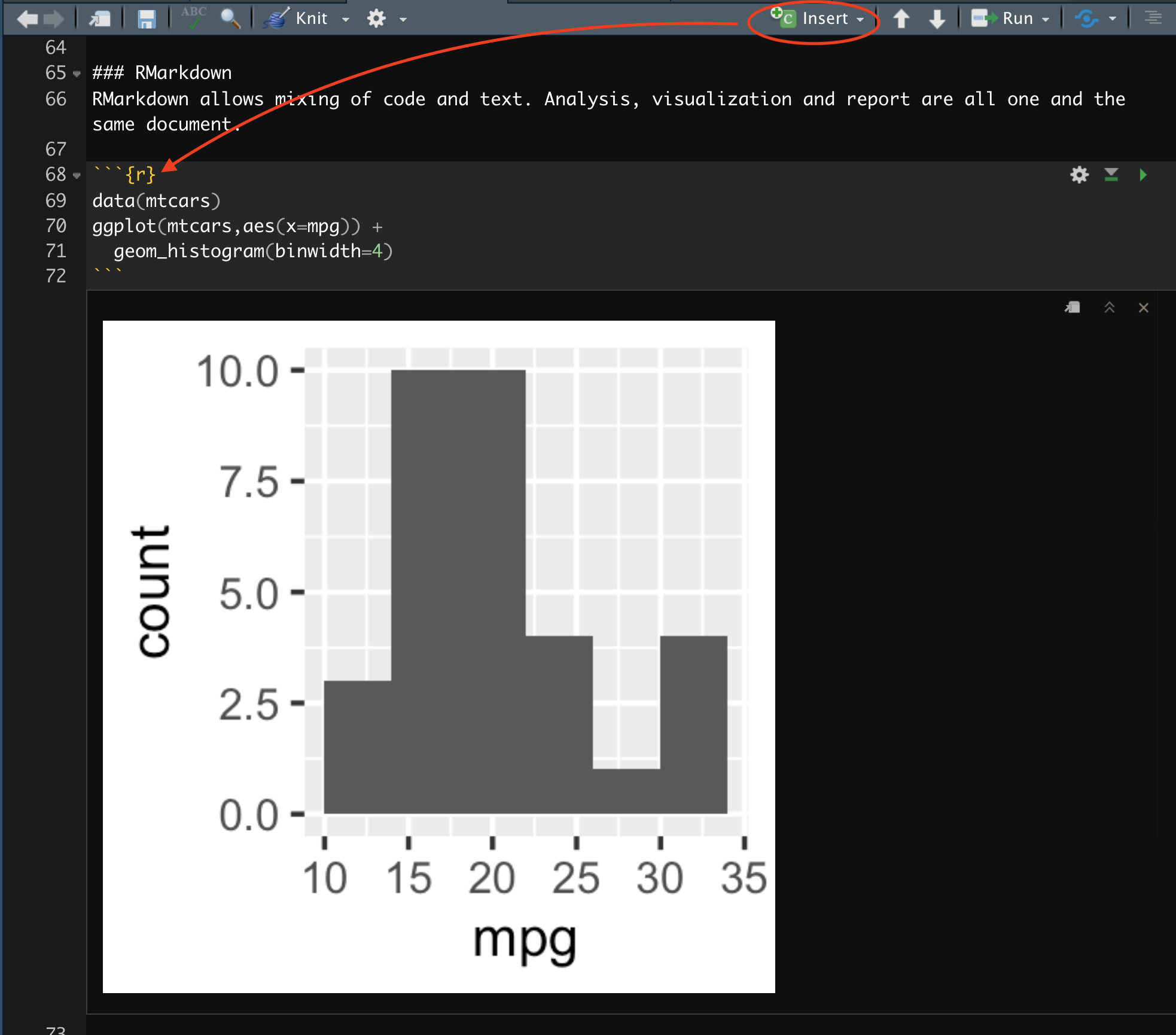
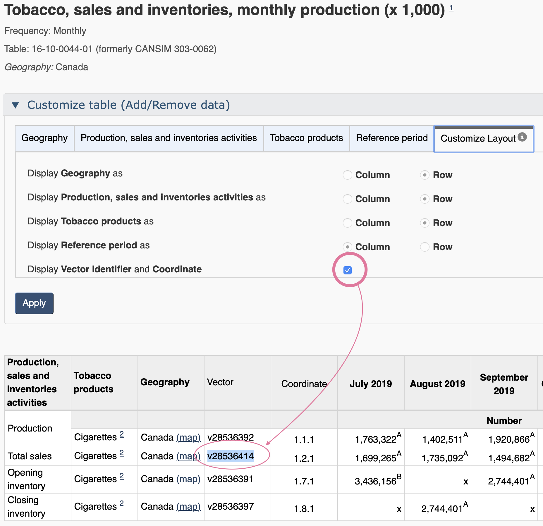
class: center, middle, inverse, title-slide

# {cansim} and Data Visualization
## CABE Workshop
### Jens von Bergmann
### 2021-03-18

---

## {cansim} and Data Visualization
Slides are at https://mountainmath.ca/cabe_workshop1 for those wanting to follow along and copy-paste code on their own machine.

StatCan data is at the base of a lot of analysis in Canada. StatCan tables (formerly CANSIM) cover current and past timelines of Canadian socio-economic data. They update regularly, which means there is a high pay-off for reproducible and adaptable workflows and analysis.

--
* **Reproducible**: can be repeated by others with minimal work, can be repeated as new data comes in (also auditable)

--
* **Adaptable**: can be easily tweaked to accomplish related tasks

--
* **Polished visualizations**: can be directly used for publication, with no (or minimal) extra work

The [*R* programming language](https://www.r-project.org). Ideally using the [RStudio IDE](https://rstudio.com). We will be working with [RMarkdown](https://bookdown.org/yihui/rmarkdown/notebook.html) documents, and need the following packages:
  - [`cansim` package](https://mountainmath.github.io/cansim/) to access census data via the [StatCan NDM API](https://www.statcan.gc.ca/eng/developers/wds)
  - [tidyverse](https://www.tidyverse.org), an *opinionated collection of R packages* for intuitive general-purpose data manipulations and visualization capabilities.

---
## Agenda

We will explore how to
* access StatCan tables data
* explore the datasets and perform basic data manipulations
* perform basic descriptive analysis and visualization

---
## Getting set up
For those wishing to follow along live-coding, open a new RMarkdown document.

.pull-left[
![](images/open_rmarkdown.png)
]
.pull-right[
![](images/open_rmarkdown2.png)
]

---
.pull-left[

### RMarkdown
RMarkdown allows mixing of code and text. Analysis, visualization and report are all one and the same document.

```r
library(tidyverse)
data(mtcars)
ggplot(mtcars,aes(x=mpg)) + 
  geom_histogram(binwidth=4)
```

![](cabe_workshop1_files/figure-html/unnamed-chunk-1-1.svg)

]
.pull-right[
![](images/open_rmarkdown3.png)

RMarkdown documents can be compiled to **HTML**, **PDF** or **Word**.

The output of code blocks gets inserted into the document. We can show or hide the actual code.

These slides are entirely done in RMarkdown.
]
---
# cansim
.pull-left[
The [`cansim` R package](https://mountainmath.github.io/cansim/) interfaces with the StatCan NDM that replaces the former CANSIM tables. It can be queried for
- whole tables
- specific vectors
- data discovery searching through tables

It encodes the metadata and allows to work with the internal hierarchical structure of the fields.

```r
#install.packages("tidyverse")
library(tidyverse)
#install.packages("cansim")
library(cansim)
```
]
.pull-right[
<img src="https://raw.githubusercontent.com/mountainMath/cansim/master/images/cansim-sticker.png" alt="cansim" style="height:500px;margin-top:-80px;">
]

---
## First example: Motor vehicle sales
To start off we grab data on motor vehicle sales from table 20-10-0001 and inspect the available variables.

```r
mv_sales <- get_cansim("20-10-0001") %>%
  normalize_cansim_values(factors=TRUE)

mv_sales %>% select_if(is.factor) %>% lapply(levels)
```

```
## $`Vehicle type`
## [1] "Total, new motor vehicles" "Passenger cars"            "Trucks"                   
## 
## $`Origin of manufacture`
## [1] "Total, country of manufacture" "North America"                 "Total, overseas"              
## [4] "Japan"                         "Other countries"              
## 
## $Sales
## [1] "Units"   "Dollars"
## 
## $`Seasonal adjustment`
## [1] "Unadjusted"          "Seasonally adjusted"
```

---
## Motor vehicle sales (Notes)
It's always good to check the notes so there are no unexpected hiccups.
.medium-font[

```r
get_cansim_table_notes("20-10-0001") %>%
  knitr::kable()
```

|Dimension name        |Note ID |Member Name                          |Note                                                                                                                                |
|:---------------------|:-------|:------------------------------------|:-----------------------------------------------------------------------------------------------------------------------------------|
|NA                    |1       |NA                                   |Prior to 1953, data for Canadian and United States manufactured vehicles and overseas manufactured vehicles are not segregated.     |
|Geography             |2       |British Columbia and the Territories |Includes Yukon, Northwest Territories and Nunavut.                                                                                  |
|Vehicle type          |3       |Trucks                               |Trucks include minivans, sport-utility vehicles, light and heavy trucks, vans and buses.                                            |
|Origin of manufacture |4       |Total, overseas                      |Includes Japan and other countries.                                                                                                 |
|Seasonal adjustment   |5       |NA                                   |Seasonally adjusted data for the New Motor Vehicle Sales survey are available for the period between January 1991 to February 2012. |
]

We take note of the definition for **Trucks** and that **seasonally adjusted** data has been discontinued.

---
## Motor vehicle sales

```r
plot_data <- mv_sales %>% 
  filter(GEO=="Canada",
         Date>=as.Date("1990-01-01"),
         `Vehicle type`!="Total, new motor vehicles",
         `Origin of manufacture`=="Total, country of manufacture",
         Sales=="Units",
         `Seasonal adjustment`=="Unadjusted")

ggplot(plot_data,aes(x=Date,y=VALUE,color=`Vehicle type`)) +
  geom_line() 
```

![](cabe_workshop1_files/figure-html/unnamed-chunk-5-1.svg)

---
## Motor vehicle sales (nicer graph)

```r
g <- ggplot(plot_data, aes(x=Date,y=VALUE,color=`Vehicle type`)) +
  theme_light() +
  geom_line(alpha=0.2) + 
  geom_smooth(span=0.1) + 
  scale_y_continuous(labels=function(d)scales::comma(d,scale=1/1000,suffix="k")) +
  labs(title="Canadian new motor vehicle sales",x=NULL,y="Sales per month",
       caption="StatCan Table 20-10-0001")
g
```

![](cabe_workshop1_files/figure-html/unnamed-chunk-6-1.svg)

---
class: medium-code
## Motor vehicle sales (annotated graph, final version)

```r
library(ggrepel)   # (for nicer labels)
g + geom_text_repel(data=~filter(.,Date==as.Date("1990-08-01"),`Vehicle type`=="Passenger cars"),
                   label="Passenger cars",hjust=0,nudge_y = 30000) +
  geom_text_repel(data=~filter(.,Date==as.Date("2016-11-01"),`Vehicle type`=="Trucks"),
                   label="Trucks, SUVs, Vans, Buses",
                  hjust=1,nudge_x = -2000,nudge_y=10000) +
  scale_color_manual(values=c("Passenger cars"="steelblue","Trucks"="brown"),guide=FALSE)
```

![](cabe_workshop1_files/figure-html/unnamed-chunk-7-1.svg)

---
class: medium-code
## Motor vehicle sales (seasonality)

```r
plot_data %>% rename(type=`Vehicle type`) %>%
  ggseas::ggsdc(aes(x=Date,y=VALUE,color=type),method="stl",frequency = 12,s.window = 24) +
  theme_light() + geom_line() + 
  scale_color_manual(values=c("Passenger cars"="steelblue","Trucks"="brown"),guide=FALSE) +     
  scale_y_continuous(labels=function(d)scales::comma(d,scale=1/1000,suffix="k")) +
  labs(title="Canadian new motor vehicle sales (STL decomposition)",x=NULL,y="Sales per month",
       colour = "Vehicle type",caption="StatCan Table 20-10-0001")
```

![](cabe_workshop1_files/figure-html/unnamed-chunk-8-1.svg)

---
class: medium-code
## Building permits
A more complex example.

```r
permit_data <- get_cansim("34-10-0066") %>% 
  normalize_cansim_values(factors=TRUE)

permit_data %>% select_if(is.factor) %>% sapply(function(c)levels(c) %>% length)
```

```
##   Type of structure        Type of work           Variables Seasonal adjustment 
##                  89                  22                   5                   2
```

There are a lot of different categories! Let's inspect some.

```r
permit_data$Variables %>% levels
```

```
## [1] "Value of permits"                    "Number of dwelling-units created"    "Number of dwelling-units lost"      
## [4] "Number of dwelling-units demolished" "Number of permits"
```

```r
permit_data$`Type of work` %>% levels %>% head()
```

```
## [1] "Types of work, total"                                     "New dwelling units total"                                
## [3] "New residential and non-residential constructions, total" "New construction"                                        
## [5] "Foundation"                                               "Superstructure or part of a new building"
```
---
class: medium-code
## Filtering and summarizing
We filter down the categories we are interested in and inspect the result.

```r
permits <- permit_data %>%
  filter(`Type of structure` %in% c("Total residential","Total demolitions"),
         `Type of work`== "Types of work, total",
         `Seasonal adjustment`=="Unadjusted") %>%
  filter(grepl("Toronto|Vancouver|Montr|Calgary",GEO)) %>%
  select(GEO,Date,Variables,VALUE)

tail(permits)
```

```
## # A tibble: 6 x 4
##   GEO                         Date       Variables                               VALUE
##   <chr>                       <date>     <fct>                                   <dbl>
## 1 Calgary, Alberta            2021-01-01 Number of dwelling-units demolished        19
## 2 Vancouver, British Columbia 2021-01-01 Value of permits                    406753000
## 3 Vancouver, British Columbia 2021-01-01 Number of dwelling-units created         1610
## 4 Vancouver, British Columbia 2021-01-01 Number of dwelling-units lost               1
## 5 Vancouver, British Columbia 2021-01-01 Number of permits                         589
## 6 Vancouver, British Columbia 2021-01-01 Number of dwelling-units demolished       153
```
---
class: medium-code
## Reshaping the data
The data we have is in **long form**, we reshape the *Variables* column to **wide form** to more easily perform calculations.
.medium-font[

```r
plot_data <- permits %>%
  pivot_wider(names_from=Variables,values_from = VALUE) %>%
  mutate(ratio=(`Number of dwelling-units lost`+`Number of dwelling-units demolished`)/
           `Number of dwelling-units created`)

plot_data %>% select(matches("Date|GEO|Number of dw")) %>% tail() %>% knitr::kable()
```

|GEO                         |Date       | Number of dwelling-units created| Number of dwelling-units lost| Number of dwelling-units demolished|
|:---------------------------|:----------|--------------------------------:|-----------------------------:|-----------------------------------:|
|Calgary, Alberta            |2020-12-01 |                              577|                             0|                                  28|
|Vancouver, British Columbia |2020-12-01 |                             2299|                             3|                                 193|
|Montréal, Quebec            |2021-01-01 |                             1917|                            27|                                 101|
|Toronto, Ontario            |2021-01-01 |                             5949|                             6|                                  79|
|Calgary, Alberta            |2021-01-01 |                             1270|                             0|                                  19|
|Vancouver, British Columbia |2021-01-01 |                             1610|                             1|                                 153|
]
---
class: medium-code
## Units lost per units created

```r
ggplot(plot_data,aes(x=Date,y=ratio)) +
  geom_bar(stat="identity",fill="steelblue") +
  facet_wrap("GEO",nrow=1) +
  geom_smooth(formula=y~1,method="lm",se=FALSE,color="brown") +
  labs(title="Dwelling units lost/demolished per unit created",x=NULL,y=NULL,
       caption="StatCan Table 34-10-0066") 
```

![](cabe_workshop1_files/figure-html/unnamed-chunk-14-1.svg)

---

## Cigarette sales
.pull-left[
Sometimes we are just interested in one specific variable. It can be easier to pull in the StatCan vector.

Vector discovery can be cumbersome, downloaded table data has it. The web view has it too.

We can go to the web view of table right from the R console using the following command.

```r
view_cansim_webpage("16-10-0044")
```

Selecting the **Add/Remove data** option allows us to filter the data down to what we want and enable the display of StatCan vectors.
]

.pull-right[
![](images/cigarette_sales.png)
]
---
class: medium-code
## Cigarette sales

```r
g <- get_cansim_vector("v28536414","1800-01-01") %>% 
  normalize_cansim_values() %>%
  ggplot(aes(x=Date,y=VALUE)) +
  geom_line() +  geom_smooth(span=0.25,se=FALSE) +
  scale_y_continuous(labels=function(d)scales::comma(d,scale = 10E-9,suffix="bn")) +
  labs(title="Canadian cigarette sales",x=NULL,y="Monthly sales",caption="StatCan vector v28536414")
g
```

![](cabe_workshop1_files/figure-html/unnamed-chunk-16-1.svg)

---
class: medium-code
## Cigarette sales (adding context)

```r
g + 
  geom_vline(xintercept = as.Date(c("2005-03-18","2005-08-22","2006-05-31","2006-12-01",
                                    "2007-01-01","2007-06-17","2010-07-05","2012-02-22")),
             linetype="dashed", color="brown") +
  geom_label(x=as.Date("2010-01-01"),y=3.3E9,label="Partial smoking bans\nand advertising limitations", 
            hjust=0.5,color="brown") +
  geom_label(x=as.Date("2020-08-01"),y=2.5E9, label="No visible impact\nof COVID-19", hjust=0.8)
```

![](cabe_workshop1_files/figure-html/unnamed-chunk-17-1.svg)

---
class: medium-code
## Housing consumption share of GDP
Sometimes we need more data processing to get to quantities we are interested in.

```r
gdp_data <- get_cansim("36-10-0402") %>% 
  normalize_cansim_values(factors="true") %>%
  filter(Value=="Chained (2012) dollars") %>%
  select(Date,GEO,naics=`North American Industry Classification System (NAICS)`,VALUE)
```
We already cut down to Chained (2012) dollars for units, and cleaned up the data and simplified the names.

```r
head(gdp_data)
```

```
## # A tibble: 6 x 4
##   Date       GEO                       naics                                             VALUE
##   <date>     <chr>                     <fct>                                             <dbl>
## 1 1997-01-01 Newfoundland and Labrador All industries [T001]                       18691600000
## 2 1997-01-01 Newfoundland and Labrador Goods-producing industries [T002]            6353500000
## 3 1997-01-01 Newfoundland and Labrador Service-producing industries [T003]         10861000000
## 4 1997-01-01 Newfoundland and Labrador Industrial production [T010]                 4166800000
## 5 1997-01-01 Newfoundland and Labrador Non-durable manufacturing industries [T011]   576100000
## 6 1997-01-01 Newfoundland and Labrador Durable manufacturing industries [T012]       120000000
```

---
class: medium-code
## Computing shares
One frequent pattern is that we want to look at percent shares of a total. If the total is one of our columns, we can join it onto the data.

.medium-font[

```r
gdp_data_with_total <- gdp_data %>%
  left_join(filter(.,grepl("T001",naics)) %>% select(Date,GEO,Total=VALUE),
            by=c("GEO","Date")) %>%
  mutate(Share=VALUE/Total)

head(gdp_data_with_total %>% select(-GEO,-Date))
```

```
## # A tibble: 6 x 4
##   naics                                             VALUE       Total   Share
##   <fct>                                             <dbl>       <dbl>   <dbl>
## 1 All industries [T001]                       18691600000 18691600000 1      
## 2 Goods-producing industries [T002]            6353500000 18691600000 0.340  
## 3 Service-producing industries [T003]         10861000000 18691600000 0.581  
## 4 Industrial production [T010]                 4166800000 18691600000 0.223  
## 5 Non-durable manufacturing industries [T011]   576100000 18691600000 0.0308 
## 6 Durable manufacturing industries [T012]       120000000 18691600000 0.00642
```
]

---
class: medium-code
## Inspecting NAICS 53 subcodes
We are interested in real estate consumption, so we look through the real-estate realated NAICS codes.

```r
gdp_data_with_total %>% filter(grepl("\\[53",naics)) %>% pull(naics) %>% unique
```

```
##  [1] Real estate and rental and leasing [53]                                                                                                  
##  [2] Real estate [531]                                                                                                                        
##  [3] Lessors of real estate [5311]                                                                                                            
##  [4] Owner-occupied dwellings [5311A]                                                                                                         
##  [5] Offices of real estate agents and brokers and activities related to real estate [531A]                                                   
##  [6] Rental and leasing services [532]                                                                                                        
##  [7] Automotive equipment rental and leasing [5321]                                                                                           
##  [8] Rental and leasing services (except automotive equipment) [532A]                                                                         
##  [9] Lessors of non-financial intangible assets (except copyrighted works) [533]                                                              
## [10] Rental and leasing services (except automotive equipment) and lessors of non-financial intangible assets (except copyrighted works) [53A]
## 337 Levels: All industries [T001] Goods-producing industries [T002] ... Retail trade (except unlicensed cannabis) [4AZ]
```

We want subcodes starting with **5311** for rent (*Lessors of real estate [5311]*) and imputed rent (*Owner-occupied dwellings [5311A]*).

---
## Housing consumption

```r
housing_consumption <- gdp_data_with_total %>% 
  filter(grepl("5311",naics)) %>%
  group_by(Date,GEO) %>%
  summarize(Share=sum(Share)) %>%
  mutate(highlight=GEO %in% c("British Columbia","Alberta","Ontario","Quebec"))
```

We compute the combined share of those two categories for each Date and Geography.
.medium-font[

```r
head(housing_consumption)
```

```
## # A tibble: 6 x 4
## # Groups:   Date [1]
##   Date       GEO                        Share highlight
##   <date>     <chr>                      <dbl> <lgl>    
## 1 1997-01-01 Alberta                   0.0693 TRUE     
## 2 1997-01-01 British Columbia          0.132  TRUE     
## 3 1997-01-01 Manitoba                  0.111  FALSE    
## 4 1997-01-01 New Brunswick             0.0922 FALSE    
## 5 1997-01-01 Newfoundland and Labrador 0.0798 FALSE    
## 6 1997-01-01 Northwest Territories     0.0892 FALSE
```
]

---
class: medium-code
## Housing consumption share of GDP

```r
ggplot(housing_consumption,aes(x=Date,y=Share,group=GEO)) +
  geom_line(color="grey") + 
  geom_line(data=~filter(.,highlight),aes(color=GEO)) +
  theme_light() + 
  scale_y_continuous(labels=scales::percent) +
  labs(title="Housing consumption as share of GDP",caption="StatCan Table 36-10-0402",fill=NULL,x=NULL)
```

![](cabe_workshop1_files/figure-html/unnamed-chunk-24-1.svg)

---
class: medium-code
## Data discovery
Data discovery is still a major issue. Right now we have two ways

* Google
* cumbersome overview table from Open Data Canada
.medium-font[

```r
search_cansim_tables("job vacancy") %>% select(cansim_table_number,title) %>%  knitr::kable()
```

|cansim_table_number |title                                                                                                                                                   |
|:-------------------|:-------------------------------------------------------------------------------------------------------------------------------------------------------|
|14-10-0371          |Job vacancies, payroll employees, and job vacancy rate by provinces and territories, monthly, unadjusted for seasonality                                |
|14-10-0372          |Job vacancies, payroll employees, and job vacancy rate by industry sector, monthly, unadjusted for seasonality                                          |
|14-10-0326          |Job vacancies, payroll employees, job vacancy rate, and average offered hourly wage by industry sector, quarterly, unadjusted for seasonality           |
|14-10-0325          |Job vacancies, payroll employees, job vacancy rate, and average offered hourly wage by provinces and territories, quarterly, unadjusted for seasonality |
|14-10-0225          |Job vacancies, labour demand and job vacancy rate, annual, inactive                                                                                     |
|14-10-0224          |Job vacancies, labour demand and job vacancy rate, three-month moving average, unadjusted for seasonality, inactive                                     |
]

StatCan is working on better data discovery, hopefully things will get easier in the future.

---
class: medium-code
## Combining StatCan tables
To understand growth of jobs we combined LFS employment data with JVWS data on job vacancies.

```r
library(lubridate)
lfs_data <- get_cansim("14-10-0293") %>% normalize_cansim_values() %>%
  filter(`Labour force characteristics`=="Employment", Statistics=="Estimate")
jv_data <- get_cansim("14-10-0325") %>% normalize_cansim_values() %>% 
  mutate(Date=Date %m+% months(1)) %>%
  bind_rows(get_cansim("14-10-0371") %>% normalize_cansim_values()) %>%
  filter(Statistics=="Job vacancies") 
```

Job vacancies used to only be available quarterly, so take old job vacancy data time-shifted to the middle of the quarter and add on the new monthly data.

.medium-font[

```r
jv_data %>% filter(GeoUID=="59") %>% select(Date,GeoUID,`Job vacancies`=VALUE) %>% tail
```

```
## # A tibble: 6 x 3
##   Date       GeoUID `Job vacancies`
##   <date>     <chr>            <dbl>
## 1 2019-08-01 59              106260
## 2 2019-11-01 59               90140
## 3 2020-02-01 59               93125
## 4 2020-10-01 59               91705
## 5 2020-11-01 59               80115
## 6 2020-12-01 59               78680
```
]

---
class: medium-code
## Joining the two data series
The time series are collected with different frequencies, we want to only look at series where they match. An *inner join* will do that for us. We are also cutting down to four provinces.

```r
joined_jobs_data <- inner_join(lfs_data %>% select(Date,GeoUID,GEO,Employment=VALUE),
                        jv_data %>% select(Date,GeoUID,`Job vacancies`=VALUE),
                        by=c("Date","GeoUID")) %>%
  filter(GEO %in% c("Alberta","British Columbia","Ontario","Quebec"))

tail(joined_jobs_data)
```

```
## # A tibble: 6 x 5
##   Date       GeoUID GEO              Employment `Job vacancies`
##   <date>     <chr>  <chr>                 <dbl>           <dbl>
## 1 2020-11-01 48     Alberta             2227400           50435
## 2 2020-11-01 59     British Columbia    2479300           80115
## 3 2020-12-01 24     Quebec              4259600          124920
## 4 2020-12-01 35     Ontario             7299100          185430
## 5 2020-12-01 48     Alberta             2221800           35625
## 6 2020-12-01 59     British Columbia    2493500           78680
```

We now have one table with both, filled and vacant jobs, for all regions and dates for which we have data on both.

---
class: medium-code
## Reshaping the data
This time we are going to reshape the data from *wide* to *long* format. This is what makes it easiest to plot.

```r
jobs_data <- joined_jobs_data %>%
  pivot_longer(c("Job vacancies","Employment"), names_to="Type",values_to="Jobs") %>%
  mutate(Type=factor(Type,levels=c("Job vacancies","Employment")))

tail(jobs_data)
```

```
## # A tibble: 6 x 5
##   Date       GeoUID GEO              Type             Jobs
##   <date>     <chr>  <chr>            <fct>           <dbl>
## 1 2020-12-01 35     Ontario          Job vacancies  185430
## 2 2020-12-01 35     Ontario          Employment    7299100
## 3 2020-12-01 48     Alberta          Job vacancies   35625
## 4 2020-12-01 48     Alberta          Employment    2221800
## 5 2020-12-01 59     British Columbia Job vacancies   78680
## 6 2020-12-01 59     British Columbia Employment    2493500
```

We can now easily do a stacked bar chart plotting jobs over time for each region, stacking the filled and vacant jobs.

---
class: medium-code
## Jobs (filled and vacant)

```r
ggplot(jobs_data,aes(x=Date,y=Jobs,fill=Type)) +
  geom_bar(stat="identity") +
  facet_wrap("GEO",scales="free_y",nrow=1) +
  scale_y_continuous(labels=scales::comma) +
  labs(title="Jobs by economic region",fill=NULL,x=NULL,y=NULL,
       caption="StatCan Tables 14-10-0293, 14-10-0325, 14-10-0371")
```

![](cabe_workshop1_files/figure-html/unnamed-chunk-30-1.svg)

---
class: medium-code
## Income by age groups

```r
income_age_groups <- c("16 to 24 years", "25 to 34 years" , "35 to 44 years" , 
                       "45 to 54 years" , "55 to 64 years", "65 years and over")
income_data <- get_cansim("11-10-0239") %>%
  normalize_cansim_values(factors = TRUE) %>%
  filter(GEO=="Canada",
         Sex=="Both sexes",
         Statistics=="Median income (excluding zeros)",
         `Income source`=="Total income",
         `Age group` %in% income_age_groups) 
```
Sometimes we want to do several similar plots, it can be useful to define a custom theme.

```r
line_theme <- list(
  geom_line(),
  geom_point(data=~filter(.,Date==max(Date))),
  scale_color_brewer(palette="Dark2",guide=FALSE),
  theme_light(),
  expand_limits(x=as.Date("2025-01-01")),
  ggrepel::geom_text_repel(data=~filter(.,Date==max(Date)),hjust=-0.1,
                           color='black',direction="y",size=3),
  scale_y_continuous(labels=scales::dollar)
)
```

---
class: medium-code
## Income by age groups

```r
ggplot(income_data,aes(x=Date,y=VALUE,color=`Age group`,label=`Age group`)) +
  line_theme +
  labs(title="Median income by age group in Canada", x=NULL, y=unique(income_data$UOM),
       caption="StatCan Table 11-10-0239") 
```

![](cabe_workshop1_files/figure-html/unnamed-chunk-33-1.svg)

---
class: medium-code
## Wealth

```r
wealth_age_groups <- c("Under 35 years", "35 to 44 years" , "45 to 54 years", "55 to 64 years" , "65 years and older")
wealth_data <- get_cansim("11-10-0016") %>%
  normalize_cansim_values(factors=TRUE) %>%
  filter(GEO=="Canada",
         `Assets and debts`=="Net worth (total assets less total debt)",
         Statistics=="Median value for those holding asset or debt",
         `Economic family type`!="Economic families and persons not in an economic family",
         `Age group` %in% wealth_age_groups) %>%
  select(GEO,Date,`Age group`,`Confidence intervals`,`Economic family type`,UOM,VALUE) %>%
  pivot_wider(names_from="Confidence intervals",values_from="VALUE") 
```

Wealth data needs a bit more processing. The SFS is not that deep and confidence intervals can be large, so we want to pay attention to that. Also, the economic family type really matters, so we want to break that out.

```r
head(wealth_data)
```

```
## # A tibble: 6 x 8
##   GEO    Date       `Age group`  `Economic family type` UOM        Estimate `Lower bound of a 95% c… `Upper bound of a 95% c…
##   <chr>  <date>     <fct>        <fct>                  <chr>         <dbl>                    <dbl>                    <dbl>
## 1 Canada 1999-01-01 Under 35 ye… Economic families      2019 cons…    62500                    56100                    69500
## 2 Canada 1999-01-01 Under 35 ye… Persons not in an eco… 2019 cons…     7300                     4600                     9100
## 3 Canada 1999-01-01 35 to 44 ye… Economic families      2019 cons…   174100                   164600                   183200
## 4 Canada 1999-01-01 35 to 44 ye… Persons not in an eco… 2019 cons…    44400                    27800                    57700
## 5 Canada 1999-01-01 45 to 54 ye… Economic families      2019 cons…   338500                   307400                   363300
## 6 Canada 1999-01-01 45 to 54 ye… Persons not in an eco… 2019 cons…    77000                    51500                   103300
```

---
class: medium-code
## Wealth

```r
ggplot(wealth_data,aes(x=Date,y=Estimate,color=`Age group`,label=`Age group`)) +  
  geom_ribbon(aes(ymin=`Lower bound of a 95% confidence interval`,
                  ymax=`Upper bound of a 95% confidence interval`),fill="grey",alpha=0.3,size=0) +
  line_theme +
  facet_wrap("`Economic family type`") +
  labs(title="Median net worth by age group in Canada",x=NULL,y=unique(wealth_data$UOM),
       caption="StatCan Table 11-10-0239") 
```

![](cabe_workshop1_files/figure-html/unnamed-chunk-36-1.svg)

---
## Recap

* APIs, like StatCan NDM, make it easy to pull in data as needed. 
* scripting data processing in R (or other scripting languages) make analysis transparent, autitable and adaptable.
* simply re-run the scripts when new data becomes available.
* to collaborate just share the code, don't need to worry about sharing data and keeping data up-to-date.
* iterative process: can easily add data analysis and visualization.
* packages like **cansim** provides stability against API changes, they abstract the changes under the hood and deliver (more) stable results, and offer higher-level processing functionality.

--
* Still need to perform basic data processing steps. Common steps are:
  - filter() -- filter the data down to what you need
  - select() -- remove clutter and select the columns you need
  - group_by() %>% summarize() -- group and summarize data
  - ..._join() -- join two data series along common attributes (left_join, inner_join, ...)
  - pivot_wider() -- convert from long form to wide form
  - pivot_longer() -- conver from wide form to long form

---
class: medium-code
## Preview - Census Data & mixing data sources (including your own)

```r
get_census("CA16",regions=list(CMA="505"),geo_format="sf",level="CT",
           vectors=c(movers="v_CA16_6725",base="v_CA16_6719")) %>%
  ggplot(aes(fill=movers/base)) + geom_sf(size=0.1) + 
  mountainmathHelpers::geom_roads(color="grey") + mountainmathHelpers::geom_water() +
  coord_sf(datum = NA,ylim=c(45.2,45.6),xlim=c(-76.0,-75.4)) + 
  scale_fill_viridis_c(option = "inferno",labels=scales::percent) +
  labs(title="Ottawa/Gatineau share of population moved 2011-2016",fill=NULL,caption="StatCan Census 2016")
```

![](cabe_workshop1_files/figure-html/unnamed-chunk-37-1.svg)

---
class: inverse center
## Thanks for listening and coding along
The RMarkdown for this presentation can be [found on GitHub](https://github.com/mountainMath/presentations/blob/master/cabe_workshop1.Rmd) if anyone wants to download the code and adapt it for their own purposes.

### Please post your questions in the chat.
### .....<span class="blinking-cursor">|</span>

<hr>

You can find me on Twitter at [@vb_jens](https://twitter.com/vb_jens).

The [official documentations](https://mountainmath.github.io/cansim/index.html) has documentatino and examples for the {cansim} package.

My blog has lots of examples with code. [doodles.mountainmath.ca](https://doodles.mountainmath.ca)

In particular [examples using the {cansim} package](https://doodles.mountainmath.ca/categories/cansim/).